Deploying a cost-effective AI inference solution at scale requires optimization at every level. Buying the latest GPUs with the best raw performance is not enough: you must architect the entire system to make the most of all the available resources. Also, since resources are always finite, no matter how much budget you have, you still have to weigh the tradeoffs.

It takes a lot of work to deploy a cost-effective AI solution, from model preparation to optimizing every system and hardware along the way. Here are six inference optimization techniques to consider:

1. Model compression: While models are often trained in larger floating-point formats, such as FP32 or BF16, they can often be run without much loss of precision in smaller floating-point formats like FP8 or even in integer formats like INT8. Shrinking the data type reduces memory consumption, but also the computation intensity, enabling running models on simpler or fewer devices.

2. Parallelism and disaggregated execution: When models don’t fit on a single device and have to be run across multiple devices, techniques like pipeline and tensor parallelism have tradeoffs worth exploring. Furthermore, models don’t have to be executed fully on a single device just because they fit. Sometimes, it’s more efficient to split a model into parts, and execute each part on a different device or different device type.

3. KV-cache: Both the enabler and the bottleneck of LLMs, KV-cache has spawned new techniques for distributing and compressing this cache.

4. Batching: Instead of processing inference requests one at a time, batching groups multiple requests together and processes them simultaneously. This can dramatically improve throughput and hardware utilization.

5. Code generation: AI compilers translate AI models into hardware-specific instructions for efficient execution.

6. Scheduling: The final challenge is handling real user traffic efficiently, managing the set of resources at your disposal. Scheduling includes figuring out how to serve many models, from foundation models to not-so-popular models and fine-tuned variations.

Next, we’ll dive deeper into each of these topics, highlighting the brilliant work happening across industry and academia. We’ll explore what’s being done, and how it fits into the bigger picture of producing a holistically-optimized system for AI inference.

Optimizing AI inference isn't about finding a single silver bullet. It's about a holistic approach that considers every layer of the stack, from the numerical precision of the model's weights to the scheduling of user requests across a global fleet of servers.

The future of AI inference isn’t just about being the fastest, spending the most, or having the largest model. It’s about building smart, adaptable systems that deliver AI efficiently and cost-effectively. By embracing these optimization techniques, the industry can successfully transition from "growth at any cost" to sustainable, scalable AI for everyone.

Model compression

Models are usually trained with 16- or 32-bit floating point weights (e.g., BF16 or FP32). These higher-precision formats are needed during training because they offer a wide dynamic range of values, which is essential when one doesn’t yet know the range of each weight (that is discovered during training). However, the larger the number format is, the higher the energy and memory consumption are. For example, a multiplication in FP8 consumes up to 10x less energy than if done over FP32 (depending on the hardware specifications). INT8 multiplications are a further ~2x more efficient than FP8 (or up to 20x more than FP32). Also, weights in FP8/INT8 format occupy 4x less memory than in FP32.

The power consumption of data transfers from/to memory is even more impressive: transferring a 32-bit float from HBM (the type of memory used by most AI accelerators) consumes up to 50x more energy than an FP32 multiplication. This favors algorithms that reduce memory transfers even if at the expense of more arithmetic operations, as well as chips with data reuse capabilities that allow common operations to access HBM less often.

Given that AI accelerators are (and will always be) limited in terms of memory capacity and bandwidth, as well as power consumption, we should try to use the lowest possible number format to store the weights (to reduce memory usage and size of memory transfers), as well as to execute the model (to increase throughput and reduce power consumption).

Over the past few years, several techniques to compress models have been developed. These are lossy compression algorithms, meaning they reduce model size at the cost of a small drop in precision. Given that the techniques are now well understood and developed, the improvements in efficiency largely outweigh the small precision losses. Popular techniques for model compression include pruning, knowledge distillation, and quantization. These techniques can be used together, or individually.

Pruning consists of removing parts of the model (e.g., whole channels of a layer) that don’t contribute significantly to the model’s accuracy. This shrinks the size of the weights and removes some irrelevant computations. Pruning can be structured, removing entire components like channels or layers, or unstructured, which sparsifies the model by setting individual irrelevant weights to zero. Many AI accelerators are optimized for dense algebraic operations, and thus cannot handle sparse operations efficiently. However, even on this hardware, operations involving zeros can consume less power and generate less heat. On accelerators with native support for sparsity, these zero-value operations can be skipped entirely, leading to significant speedups.

Knowledge distillation is a training technique where a large, powerful “teacher” model guides the training of a smaller “student” model. While the specifics of each algorithm vary, the loss function measures the divergence between some outputs of the teacher and the student, e.g., intermediate activations or the final softmax outputs. The student model is trained so it minimizes this divergence. In practice, one can usually halve the size of the model without much accuracy loss, while some report up to 10x reductions with a 5 pp accuracy loss.

Finally, quantization is the most common compression technique. It consists of replacing operations over certain datatypes (e.g., BF16, FP32) with cheaper ones (e.g., INT8, FP8). Obviously, some accuracy is lost, but modern algorithms work pretty well. Quantization can be done either during training (slower, but usually more precise, as the quantization error is part of the loss function), or after training finishes (more common when retraining is not possible or too expensive). Quantization algorithms work by measuring the dynamic range of a particular set of values (e.g., a whole weight or a single channel of a weight) while executing a few sample inputs and then creating a function that maps numerical values (like weights or activations) from a large format into a smaller one.

There are many quantization techniques. Some replace the weights with their quantized versions and dequantize them as needed at run time. This has the advantage that it is easy to implement and often leads to better accuracy, but requires temporary memory at run time to hold at least one dequantized weight (in addition to the quantized version). Some chips can dequantize weights on the fly when loading them from memory, avoiding using temporary memory, which improves the performance substantially.

More advanced methods perform operations over quantized data directly. This has the advantage of performing operations over lower-precision data types, but it is a more complex process that needs calibration to bound the dynamic range of activations.

Given the extreme importance of quantization, this is an area still under heavy research. For example, we may soon see the use of more complex (non-affine) quantization functions, given that memory transfers consume more power than arithmetic operations, and thus it favors the tradeoff of doing more arithmetic operations to reduce the size of the weights.

Parallelism and Disaggregated Execution

Sometimes models don’t fit in the memory of a single device. Common solutions include offloading/stashing weights to the host’s RAM when not in use, or using multiple devices in parallel. The latter is the most commonly used technique because it gives the best performance; interacting with the host takes too much time (although fetching data from RAM can be overlapped with computation to hide the latency if there is sufficient memory on the device). Even when a model fits on a single device, one may want to use multiple devices to either increase overall throughput (because that may allow you to use a larger batch size to saturate the devices) or to reduce latency.

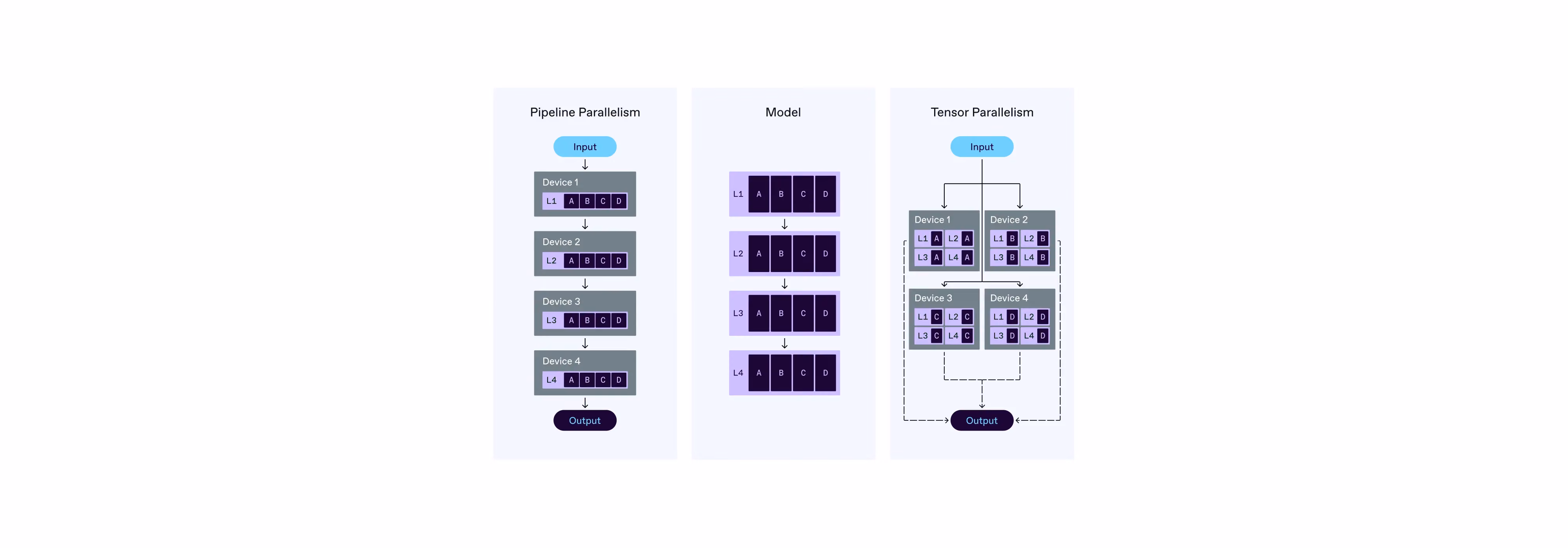
For inference, the most commonly used parallelism techniques are pipeline and tensor parallelism. They can be used individually or combined.

Pipeline parallelism works like a conveyor belt in a factory. The input comes into the first device, which runs the first few layers of the model and passes some intermediate values (activations) to the second device. This goes on until the last device, which sends the result back to the user. Pipelining increases the end-to-end latency because we now have to account for the communication between devices. On the other hand, pipelining often increases the overall throughput because each device has more space left for temporary data, which is essential to increase the batch size. Sometimes you can fit all weights in one device, but then you can’t increase the batch size enough to saturate the device. Pipelining extends the memory capacity nearly linearly with the number of devices.

In pipeline parallelism, we assign whole operations to a single device. In contrast, in tensor parallelism, we execute a single operation across multiple devices in parallel. For example, if the model performs a large matrix multiplication, we can split the matrices to execute the multiplication in a pair of devices in parallel. This effectively doubles the throughput and halves the memory consumption, both static (the weights), and dynamic (the temporary memory that matmul needs) per device as each device only handles half of the multiplication. The end-to-end latency is usually reduced due to the increase in throughput, as long as the model doesn’t require frequent synchronization between devices.

Devices need to synchronize whenever we have an operation that requires activations from the other device. This happens when two consecutive operations cannot be split in the same way (vertically, horizontally, etc.). For example, an elementwise operation followed by a reduction (like softmax) requires synchronization because reductions inherently need all the input data to produce a single output value. On the other hand, consecutive elementwise operations don’t need any synchronization, as their inputs and outputs can be sliced in the same way.

More recently, we have seen a specific kind of pipeline parallelism getting traction: E-P-D (encode-prefill-decode) model disaggregation. This consists of (manually) slicing specific layers of LLMs (E/P/D) and running each one on a different device. Again, this is just a restricted form of pipeline parallelism that is optimized for the current LLM architectures. E-P-D disaggregation was developed because there were no good automatic pipelining tools until recently, and thus deploying pipelining required a lot of manual work. We expect these special cases of pipelining to be replaced with generic pipelining as automatic tools mature.

Another emerging trend of pipelining is to use different devices for each pipeline stage. In current LLMs, the prefill phase (processing the input prompt) is compute-intensive, while the decode phase (generating output tokens one by one) is memory bound. Since there is no optimal device for every workload, it is possible to achieve a more cost-effective solution by using a heterogeneous device fleet, and use each device for what it’s best at. We expect this trend to develop further as datacenters accumulate older devices that, while they cannot run entire modern LLMs on their own, can be used effectively for some layers, extending their lifetime.

For training, there is an additional parallelization technique, popularized by DeepSpeed, that consists of sharding weights across n devices, such that each device only holds 1/n of each weight. Training usually has many replicas training on different inputs in parallel (the so-called data parallelism). Instead of duplicating the weights in each replica, this technique aims to reduce the memory consumption in an attempt to execute the model in a single device (unlike tensor parallelism, which splits weights and work across devices). The tradeoff is that it requires significant communication before each operation, where each device broadcasts its 1/n slice of the weight and receives the other n-1 slices (the so-called all-gather operation). Because this technique requires all replicas to be perfectly synchronized, this technique hasn’t seen much traction for inference workloads as it would add additional latency to collect and run the queries of hundreds of users simultaneously.

KV-Cache: The Eternal Memory/Computation Dilemma

KV-cache has become both the enabler and the bottleneck of LLMs. Before we dive into KV-cache itself, let’s refresh how current LLMs work first.

Current LLMs are based on the transformer architecture. At its core is the attention mechanism. To generate the next token (word or sub-word), the model must look back at the entire preceding sequence to understand the context. Essentially, you have a loop that produces a new token on each iteration that needs to remember the sentence that it generated so far.

Mathematically, attention is defined as:

Attention(Q, K, V) = softmax( Q · Kᵀ / √d_k ) · V

Q, K, V are each the multiplication of the input X with the respective weights (the weight matrices W are learned during training). The input X is the embeddings matrix of the sequence of tokens from the user and/or the output of a previous layer, X₁ refers to the next token being generated, and d_k is the column size of Q/K/V.

Q = X₁ · W_q​

K = X · W_k

V = X · W_v​

The most important thing to realize is that Q and X₁ are vectors with d_k columns, while K, V are matrices with dimensions (input length + tokens generated so far, d_k).

The computation time of Q is constant for each token we generate, but it is not for K and V. Their size keeps increasing as we output more tokens. The key observation is that all rows of K, V are the same for all output tokens, except that we keep appending a new row for each token. Now we have the option to recompute all of K, V for each output token, or we can cache them.

KV-cache is the name given to this cache of the intermediate K, V matrices. At each point, we retrieve the previous K, V from the cache, compute the new row, and append it.

All deployments of LLMs today use some KV-cache because it makes the attention layer linear, instead of quadratic, in the sequence length. However, KV-cache consumes a lot of memory! For example, for Llama 3.1 8B (4x more memory efficient than Llama 2), the KV-cache consumes 4 GB per user for a sequence length of 128K tokens (using FP16). For Llama 3.1 70B, the KV-Cache for 128K tokens grows to 10 GB! This is a significant percentage of any device’s memory capacity.

Because this level of memory consumption is unsustainable at scale, there is a lot of research going on to shrink the size of the KV-cache. One of the first techniques put into production is paged attention, a name that alludes to the CPUs’ memory paging mechanisms. Instead of reserving the maximum cache size for each query (e.g., allocate a 32K cache for all queries regardless of whether they will output such a long text or not), paged attention allocates the cache in pages. We could allocate each row separately, but the overhead for memory allocation would be too high. By batching allocations into pages, we reduce the time overhead of having dynamic memory allocation, at the expense of some memory being wasted at the end of the last page. One complexity of paged attention is that it requires specialized code to handle the matrices that are laid out in memory non-contiguously.

More recent work has focused on compressing the KV-cache by applying aggressive quantization. Early results suggest it is possible to shrink the KV-cache considerably with minimal impact on the accuracy. The other line of work is around distributing this cache for two purposes: simply because it may not fit into a single device, and because it can be reused across queries. For the former purpose, one can combine it with tensor parallelism to execute the attention layer in parallel across multiple devices. For the latter, one thing to realize is that many systems include system prompts, which are generic instructions prepended to each user input to restrict the behavior of the model. Instead of computing the K, V matrices for system prompts over and over again, one can precompute these and distribute them. Another simple use case is when we have users asking questions about documents or code. We can compute K, V for each document once and cache them. More advanced systems can cache K, V for common prefixes of prompts.

Memory (either HBM or SRAM) is the most expensive component we have in the datacenters today. So, expect a lot of research on shrinking the size of the KV-cache in the near future!

Batching: Escaping the Clock Frequency Wall

Current chips have a lot of computing power, but this can only be leveraged by doing a massive number of operations in parallel. Because the way we build processors hit a scaling wall two decades ago (thank you, Dennard, for your service!), we cannot increase the clock frequency anymore. As we cannot make individual operations faster, chip designers resorted to adding many arithmetic units to process operations in parallel. As a result, leveraging all this computing power requires massive parallelism in software. Current chips can perform trillions of arithmetic operations per second!

This is where batching comes in! With current LLMs, a single prompt cannot usually saturate modern chips (utilization can be as low as 10%). The solution is to execute multiple prompts in parallel. The system collects multiple requests and processes them simultaneously in a single batch to maximize hardware utilization. There are a few catches, though.

One of the concerns with batching is that it often increases the average and tail latencies. User requests don’t arrive at our servers at the same time; even in high-traffic websites, requests can be spaced a few milliseconds apart. Batching makes the first request wait for the last one, which means a few extra milliseconds of latency for the first few users. Since even millisecond-level delays can impact user engagement and revenue, balancing higher hardware utilization with strict latency targets is a critical challenge. In fact, several seminal studies have shown that even slight slowdowns decrease a website’s revenue. In summary, one needs to balance device utilization (thus cost) with the target latency.

Another important consideration is memory utilization. Remember how much memory KV-cache uses? Well, now multiply that by the batch size, and you’ll realize how quickly you run out of memory. Finding the right balance between batch size, avoiding going out of memory, and using multiple devices takes some trial and error. For example, it is not obvious when it is better to use two devices independently in a data-parallel way, or use them together using tensor parallelism to increase the batch size. Right now, there is no automatic tool that can perform such global optimizations for you.

The size of the output varies widely per prompt. The reply to some prompts can be just a “yes” or “no”, while for research prompts we may be looking at thousands of words. The problem with naive batching is that we need to execute the model for all prompts until the last one terminates. This is a lot of wasted computation, especially if the size of the output of the batched prompts differs significantly. The benefits of batching for increasing device utilization go away again. One solution is to use continuous batching. The key idea is that you don’t need to align all prompts at the beginning; you can start a prompt in the middle of the computation of another one. This can be implemented in several ways, the easiest being to pad the K,V tensors so they have the same dimension for all batches and then mask out the padded rows when computing attention. There are also specialized attention kernels for continuous batching.

One way to avoid a prompt’s output imbalance is to try to predict the sequence length and group together the requests with similar length. This way you can use the naive batching approach, which is simpler and more efficient. This strategy works only for high-traffic services, where you can have devices dedicated to specific sequence lengths.

Code Generation: Translating AI models into Assembly

So far, we’ve discussed how to optimize (compress) models and run them in parallel across multiple devices. The remaining piece of the puzzle is how models actually execute on hardware. This is where AI compilers come in: they translate AI models into hardware-specific (so-called assembly) instructions for efficient execution. Compilers are complex systems; here we give a brief overview of what goes into the compilation process.

Before starting the compilation process of an AI model, we first need to capture its dataflow graph, where vertices are algebraic operations (e.g., matrix multiplication or more complex things like softmax) and edges connect inputs and outputs of operations. Popular frameworks such as PyTorch 2 and TensorFlow expose APIs for this task. For example, one can use torch.export or torch.compile to generate the dataflow graph of a PyTorch model. The caveat is that models with data-dependent control flow (e.g., call a different function based on a value computed based on the inputs) may have multiple dataflow graphs (graph breaks in PyTorch lingo). Although frameworks now support multi-graph scenarios, the performance is still subpar. Therefore, if you want the best possible performance, avoid models with data-dependent control flow!

After capturing the dataflow graph, compilers typically apply graph-level optimizations, including removing useless operations, fusing operations together, or splitting operations apart (called lowering). The end result is a graph in the compiler’s IR (intermediate representation). Each compiler has its own IR; picking the right IR for the job is essential, and it’s a very complex decision. For example, a matrix multiplication followed by an elementwise addition (x . y + z) can be usually done together, making the addition free (since matmul is usually implemented as 0 + x . y anyway). Some IRs have a combined operation that does both operations together (like BLAS’s GEMM), while others do not. Again, the implications of these decisions are beyond the scope of this gentle introduction to AI compilers.

Fusing operations together is not just about speed, it’s also about memory. Many compilers generate code for each operation in the dataflow graph individually. This means that, for each operation, they need to load the operands from memory, execute the operation, and store the results back to memory. If the operation takes a long time to execute, the memory access time may be negligible. Otherwise, the memory access time may dominate. By fusing multiple operations, the compiler can skip materializing some intermediate results in memory and can stream them to the subsequent operation instead. Most compilers have heuristics to decide when to fuse neighboring operations, as this is one of the optimizations that yields the most speedup. For example, FlashAttention is a particular way of computing the attention layer that avoids materializing large intermediate results by computing softmax on the fly, since the result of softmax is much smaller than its input.

Another important optimization is deciding on the memory layout for each tensor, including user inputs, intermediate and temporary results, and outputs. You are probably familiar with row-major and column-major indexing orders for matrices. AI models take this complexity to the next level because tensors typically have 4 or 5 dimensions. Picking the right layout can affect the performance of an algorithm significantly, depending on the memory access patterns supported by the hardware, cache line sizes, etc. Also, many AI accelerators have HBM, SRAM, registers, etc; all of these have very different access speeds, sizes, energy consumption, and so on. The compiler must decide on the best way to slice the data across these different memories at each point in time. The compiler may also decide to replicate data into multiple memories if the replication time is offset by a faster operation execution.

We have previously discussed parallelization across devices, but parallelization within a device is also important. Current chips have many arithmetic units, and so the compiler must be able to split individual operations to take advantage of this computing power. Another important job of the compiler is to schedule operations. Sometimes it is possible to interleave computations and data transfers to hide the latency of data transfers. However, this increases the peak memory consumption, as well as the peak energy consumption (which can then reduce the power available for computations). The compiler must thus balance all of these factors.

Optimization is always relative to some metrics. Typical compiler optimization metrics include raw speed (throughput), energy efficiency, and code size. Sometimes reducing the performance only slightly (1-5%) can increase efficiency significantly. This is something that you need to account for given your performance targets and budget. Code size is often overlooked, but the code size of some models can be upwards of hundreds of MBs. This can make the difference between being able to increase the batch size or not, which is why the compiler should be mindful.

Related with metrics are the cost models. The compiler must know the impact of each decision it makes on the relevant metrics. This is called the cost model, as it models the execution cost of a program on a particular device. As devices have become more complex, it has become expensive to write accurate-enough cost models. Some compilers (e.g., Triton) use a process called auto-tuning, which consists of generating a few hundred or thousands of compiled programs, running them, and picking the best one. This avoids having to create a very precise cost model at the expense of making the compilation process slower. This process is reasonable if you are going to execute the model for a while. Some chips are deterministic and regular enough that you can specify a cost model by hand.

Some compilers do only local (greedy) optimization, i.e., they optimize each operation at a time. This process is simple and scalable; you can even compile the whole dataflow graph in parallel. The issue is that sometimes the optimal code and memory layout for an operation makes the subsequent operation much slower. This is where global optimization comes into play: it can, for example, slow down one operation slightly to make the subsequent one much faster, yielding a faster end-to-end result. FuriosaAI’s compiler is one of the few that does global optimization like this.

There are different kinds of compilers. The simplest ones usually come with a huge library with all sorts of operations implemented by hand. The compiler’s job is then to call the right sequence of library functions. The advantage of this approach is that it’s the easiest to get a device up and running. The disadvantages are: the set of models that can be run efficiently is limited by what’s implemented in the library, and thus the vendor needs to update the library for each model release; code size, since these libraries grow very large; and performance, since the opportunities for operation fusion or interoperation optimization are very limited. Building a compiler that does not use a library requires a considerably larger investment, but usually pays off in the long run, since it reduces the cost of maintaining the large library. Many compilers thus use a hybrid library/codegen approach.

Finally, compilers need to take numerical stability into account. Floating-point numbers have well-known precision problems. Some algorithms, if implemented naively, keep accumulating small errors at each step, which can then lead to catastrophic errors in the result. Although compilers have typically implemented the so-called “fast-math” mode, where floats are treated as if they were reals, AI compilers have learned over time to be more careful. No one wants a NaN as the response to their prompt!

Whole-Datacenter Optimization: Scheduling under an SLO

Once your AI model is trained and deployed, the final challenge is handling real user traffic efficiently. Whatever your budget is, the set of resources at your disposal is always going to be finite, so it is a good idea to understand how to make the most of these resources.

Service-Level Objectives (SLOs) define measurable targets for your service performance (e.g., latency, reliability), not just what you wish to achieve, but what you commit to delivering. For example, for an LLM deployment there are two common metrics: TTFT (time to first token), which measures the latency for the client to receive the first output token, and TPOT (time per output token), which measures the average time for delivering the subsequent tokens. The reason for having separate metrics is that TTFT has a direct impact on the user experience, since that’s the time the user needs to wait until some answer starts showing up on the screen. TPOT is usually lower than TTFT because there is often some overhead in starting the model execution and the first token may require more computation. SLOs may include other metrics, such as reliability (how many 9’s, e.g., the service must be up 99.9% of the time).

The metrics in SLOs are usually given in percentile. For example, a 100ms P95 for TTFT means that 95% of the users receive the first token within 100ms. Averages can hide the tail latency, so percentile metrics have become the norm.

After the SLO is written down, your job is to create the cheapest possible solution. It’s not the best idea to return the first token in 50ms if your SLO says you have 100ms. We discussed before some ways to increase efficiency at the cost of latency, namely batching and execution disaggregation (pipelining). In the other direction, there are techniques to reduce latency, especially for the first few tokens (that impact the user experience the most).

One technique to reduce latency is called speculative decoding. The key enabler is that although generation is a sequential process (remember that the attention layer needs to know the previously generated tokens), verifying if a sequence of tokens corresponds to what the model would generate can be done in parallel. The trick consists in using a smaller (draft) model to predict the first few tokens, and then use the large model to validate whether the prediction is correct. Some deployments only validate the tokens that the draft model is unsure about. This technique allows the system to produce the first few tokens for roughly the same time it would take to produce just the first token. The downside is that this process reduces the overall efficiency since now we need to run two models instead of one (if validating all tokens).

If you are resource constrained (aren’t we all?), you may want to consider a few additional tricks. If you have different traffic tiers (like free and premium), you want to have different QoS (quality of service) considerations for each tier. This may mean relaxing the SLOs so you can gracefully degrade the quality of service for the lower tiers during peak hours. For example, during peak hours you can adjust the validation threshold for the draft model when running speculative decoding for non-premium traffic (so it trusts the draft model more and thus validates less). You may even switch the lower tiers to smaller models altogether. You may also want to increase the batch size if there is still room to increase efficiency that way.

This area of model serving is still in very early days, with research starting to scratch the surface right now. We now speculate about some areas where we expect to see developments in the near future. One area is around hardware bidding. Some cloud providers allow you to bid for VMs that are otherwise idle. The prices are quite competitive (up to 10x cheaper than regular instances), so it makes sense to take advantage of these resources. We expect to see load balancers that can predict traffic patterns and proactively bid for VMs of different cloud providers. This system can be aware of the geographic distance between devices and traffic origin, such that it understands that it can get a device further away as long as it is fast enough to compensate for the extra network latency. This kind of load balancer will be able to do global optimization, delivering the most cost-effective solution that meets the SLOs, while doing graceful service degradation or even reject traffic if the cost reaches some threshold or if it runs out of resources.

Another area to watch is around sharing parts of fine-tuned models. Some inference-as-a-service providers now face a “tail model” problem: they host a vast number of models, but many of them (the "long tail") receive infrequent traffic. This makes it inefficient to keep them loaded on a dedicated accelerator all the time. The issue is that context-switching the weights between the device memory and the host’s RAM takes too long. We expect to see further work on sharing parts of models, especially between variants of a model that were fine-tuned to specific tasks, to increase the number of models that can be served per device. Most recent work focuses on variants of LoRA (low-rank adaptation).